Legged Robot Basic Knowledge
[TOC]
0 序言
从本科开始,我就对会走的机器人十分感兴趣,好奇通过什么样的控制可以使其运动起来。在2014年的时候,我就制作了舵机驱动的四足机器人,每条腿4个自由度。不过由于舵机的输出力较小,我设计的结构也不够优化,机器人只能踉踉跄跄的走两步,远达不到动态控制的目标。那个时候我只能自己研究,连 《Legged Robots That Balance 》1这样经典的资料都没有看过。后来我又折腾过很多其他的杂七杂八的小玩意,直到读研究生的时候,才又开始研究四足机器人的控制问题。那时候刚好是2018年,是MIT Cheetah火起来的时候。从那以后,我断断续续的持续积累着相关知识,因此想总结一下,方便我后续的学习与工作,也希望可以借此和其他人一起交流进步。我的邮箱是759094438@qq.com,如果有错误疏漏或者是相关问题,欢迎发邮件一起讨论。在这里我参考了许多人的资料2,后续会一一列举,如有遗漏,也请补充指正。
——2024年1月
1 足式机器人建模
首先,第一部分是对足式机器人进行理论建模,方便后续的各种分析。这里的基本参考资料是《Modern Robotics: Mechanics, Planning, and Control》3,这本书有中文版,是北航的于靖军教授翻译的,是十分优秀的入门教材。如果单纯想深入学习一下背后的旋量理论,可以参考《机构学与机器人学的几何基础与旋量代数》4,写的简明易懂,没有过于艰涩的数学内容。还有就是《Springer Handbook of Robotics, Second Edition》5是很全面的参考手册,需要哪个部分的知识去对应章节查询即可。
如果想要深入研究足式机器人运动控制算法背后的数学原理,我推荐CMU Zachary Manchester的Optimal Control6的课程进行进一步学习。该课程相关的参考书有《Nonlinear programming》7《Reinforcement Learning and Optimal Control》8《Numerical Optimization, Second Edition》9《Practical Methods for Optimal Control and Estimation Using Nonlinear Programming》10。其中,《Numerical Optimization, Second Edition》9是对课程里面优化算法的一个很好的补充资料,书里面有很多图便于理解,也没有很多复杂的数学证明过程,对实际应用比较友好。
1.1 正运动学(Forward Kinematics)
正运动学是在已知机器人构型和机器人关节角度后,得到机器人末端位置的一种方法。机器人构型主要分为串联机器人、并联机器人和串并联机器人。串联机器人的正运动学可以直接得到解析解,很好计算。并联机器人的正运动学很难得到解析解,很可能用数值方法才能求解。串并联机器人的求解难度适中,大体按照串联机器人的方法计算,仅针对其中的部分并联关节特殊处理。
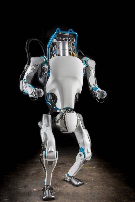
为了方便理解,我在网上找了两个机器人的机构示意图。不同的机器人结构都有所区别,但是基本的计算原理是一样的。人形机器人的结构示意图11如下图所示:
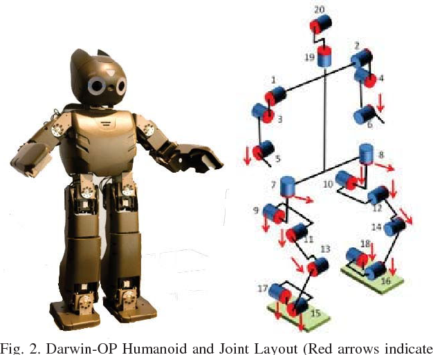
人形机器人结构示例
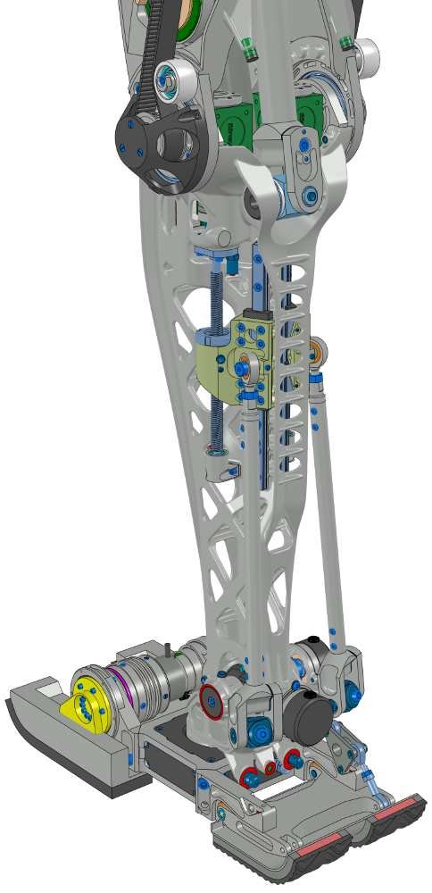
四足机器人的结构示意图12如下图所示:
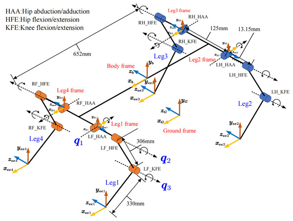
四足机器人结构示例
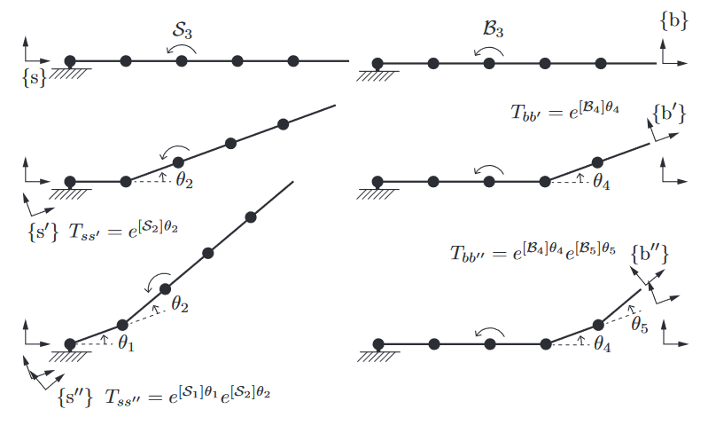
这两种机器人的正运动学分析都很简单,均可通过《Modern Robotics: Mechanics, Planning, and Control》3里的旋量方法进行建模。具体来说,需要手臂或者是腿在所有关节位置为0的状态下,末端在身体坐标系的初始位姿矩阵 $ M $ 和 每个轴的旋量 $ \bold{S}_i 或\bold{B}_i $表示,然后通过指数运算公式得到指定关节位置 $ \bold{q}=[\theta_1, \theta_2 … \theta_N] $ 的情况下的末端位置。
\begin{equation} \begin{aligned} T = e^{[\bold{S_1}]\theta_1}e^{[\bold{S_2}]\theta_2}...e^{[\bold{S_N}]\theta_N}M \end{aligned} \end{equation}
\begin{equation} \begin{aligned} T = Me^{[\bold{B_1}]\theta_1}e^{[\bold{B_2}]\theta_2}...e^{[\bold{B_N}]\theta_N} \end{aligned} \end{equation}
1.2 逆运动学(Inverse Kinematics)
逆运动学是已经得知机器人末端的位姿后,求解关节位置 $\bold{q}=[\theta_1, \theta_2 … \theta_N] $的方法。串联机器人的求解较为困难,可以使用Newton方法及其变种来在实际应用中快速求解,而并联机器人大部分可以直接得到解析解。串并联机器人的逆运动学计算基本方法是按照串联机器人进行,针对并联的关节特殊处理。
四足机器人的腿部结构样式比较少,现在流行的大部分结构就如同上一节的图片所示,这样的结构也很方便逆运动学求解。对XYZ三个轴向分别投影,按照几何关系很容易求解。而人形机器人或者是双足机器人的结构就比较多种多样,下面是几种常见的机器人结构,包括3自由度腿13、5自由度腿14、串并联的结构(并联踝关节)1516等:
人形机器人示例
def IKinSpace(Slist, M, T, thetalist0, eomg, ev):
    thetalist = np.array(thetalist0).copy()
    i = 0
    maxiterations = 20
    Tsb = FKinSpace(M, Slist, thetalist)
    Vs = Adjoint(Tsb) @ se3ToVec(MatrixLog6(TransInv(Tsb) @ T))
    err = np.linalg.norm([Vs[0], Vs[1], Vs[2]]) > eomg or np.linalg.norm([Vs[3], Vs[4], Vs[5]]) > ev
    while err and i < maxiterations:
        thetalist = thetalist + np.linalg.pinv(JacobianSpace(Slist, thetalist)) @ Vs
        i = i + 1
        Tsb = FKinSpace(M, Slist, thetalist)
        Vs = Adjoint(Tsb) @ se3ToVec(MatrixLog6(TransInv(Tsb) @ T))
        err = np.linalg.norm([Vs[0], Vs[1], Vs[2]]) > eomg or np.linalg.norm([Vs[3], Vs[4], Vs[5]]) > ev
    return (thetalist, not err)
为了提高效率与保证数值稳定性,Newton-Raphson还有很多变种,包括使用伪逆代替直接求逆、对每次的更新量添加\lambda的damping(相当于非常简易的Line Search)来避免求解震荡、以及UCLA使用的Damped Least Squares的方法17,如下所示。这些求解逆运动学的数值方法都很快,一般在5次迭代内就可以收敛,可以用于实际的实时机器人控制。
def IKinSpaceDampedLeastSquare(Slist, M, T, thetalist0, lamb, W, eomg, ev):
    thetalist = np.array(thetalist0).copy()
    i = 0
    maxiterations = 20
    Tsb = FKinSpace(M, Slist, thetalist)
    Vs = Adjoint(Tsb) @ se3ToVec(MatrixLog6(TransInv(Tsb) @ T))
    err = np.linalg.norm([Vs[0], Vs[1], Vs[2]]) > eomg or np.linalg.norm([Vs[3], Vs[4], Vs[5]]) > ev
    while err and i < maxiterations:
        J = JacobianSpace(Slist, thetalist)
        JJT = J.T @ W @ J + lamb * np.eye(thetalist.size)
        thetalist = thetalist + np.linalg.pinv(JJT) @ J.T @ W @ Vs
        i = i + 1
        Tsb = FKinSpace(M, Slist, thetalist)
        Vs = Adjoint(Tsb) @ se3ToVec(MatrixLog6(TransInv(Tsb) @ T))
        err = np.linalg.norm([Vs[0], Vs[1], Vs[2]]) > eomg or np.linalg.norm([Vs[3], Vs[4], Vs[5]]) > ev
    return (thetalist, not err)
1.2.1 高擎机电双足机器人运动学分析
本小节针对一款实际的人形机器人进行运动学分析,并给出对应的python代码。根据《Modern Robotics: Mechanics, Planning, and Control》一书,旋量的定义为:
\begin{equation}
\begin{aligned}
\bold{S} =
\begin{bmatrix}
\bold{\omega} \\ \bold{v}
\end{bmatrix} =
\begin{bmatrix}
\hat{\bold{s}} \\ -\hat{\bold{s}} \times \bold{q} + h\hat{\bold{s}}
\end{bmatrix}
\end{aligned}
\end{equation}
其中,\hat{\bold{s}}是指关节轴的方向,q为关节轴上一点的坐标,h为螺旋轴节距,对于1-DOF纯旋转关节来说,h=0。所以可以得到腿部所有关节的旋量:
\begin{equation}
\begin{aligned}
\bold{S_1} =
\begin{bmatrix}
1 \\ 0 \\ 0 \\ 0 \\ 0 \\0
\end{bmatrix},
\bold{S_2} =
\begin{bmatrix}
0 \\ 0 \\ 1 \\ 0 \\ 0 \\0
\end{bmatrix},
\bold{S_3} =
\begin{bmatrix}
0 \\ 1 \\ 0 \\ 0 \\ 0 \\0
\end{bmatrix},
\bold{S_4} =
\begin{bmatrix}
0 \\ 1 \\ 0 \\ L_1 \\ 0 \\0
\end{bmatrix},
\bold{S_5} =
\begin{bmatrix}
0 \\ 1 \\ 0 \\ L_1 + L_2 \\ 0 \\0
\end{bmatrix}
\end{aligned}
\end{equation}
其中,L_1和L_2为大腿和小腿的长度。腿的初始位姿矩阵M为:
\begin{equation}
\begin{aligned}
M=
\begin{bmatrix}
1 & 0 & 0 & 0 \\
0 & 1 & 0 & 0 \\
0 & 0 & 1 & -(L_1 + L_2 + L_3) \\
0 & 0 & 0 & 1
\end{bmatrix}
\end{aligned}
\end{equation}
随后可以用下述公式求解正运动学:
\begin{equation}
\begin{aligned}
T = e^{[S_1]\theta_1}e^{[S_2]\theta_2}...e^{[S_N]\theta_N}M
\end{aligned}
\end{equation}
对应的python代码18如下:
def FKinSpace(M, Slist, thetalist):
    T = np.array(M)
    for i in range(len(thetalist) - 1, -1, -1):
        T = MatrixExp6(VecTose3(np.array(Slist)[:, i] * thetalist[i])) @ T
    return T
对于逆运动学,采用了数值方法,没有使用解析解的方法,采用的是上一节提到的IKinSpaceDampedLeastSquare函数,在运行时,通常可以在3-4个循环中求出关节逆解,对应的仿真代码可以参考18。
高擎机电双足机器人
1.3 雅可比矩阵
从前面的描述,我们可以知道,关节的末端位姿是关节角度的函数,可以表示为:
\begin{equation} \begin{aligned} \bold{x}=f(\bold{q}) \end{aligned} \end{equation}
想要得到末端的速度,那么我们可以对上面的函数求导,结合链式法则可以得到:
\begin{equation}
\begin{aligned}
\dot{\bold{x}}=
\frac{\partial f(\bold{q})}{\partial \bold{q}} \frac{d\bold{q}}{dt} =
\frac{\partial f(\bold{q})}{\partial \bold{q}} \dot{\bold{q}} = J(\bold{q}) \dot{\bold{q}}
\end{aligned}
\end{equation}
其中,J(\bold{q}) \in \mathbb{R}^{m \times n}即为雅可比矩阵(Jacobian)。把这个公式代入对正运动学的公式求导,可得:
\begin{equation}
\begin{aligned}
\dot{T} =
(\frac{\mathrm{d}}{\mathrm{d}t} e^{[\bold{S_1}]\theta_1}) \dots e^{[\bold{S_n}]\theta_n} M + e^{[\bold{S_1}]\theta_1}(\frac{\mathrm{d}}{\mathrm{d}t} e^{[\bold{S_2}]\theta_2}) \dots e^{[\bold{S_n}]\theta_n} M + \dots + e^{[\bold{S_1}]\theta_1} \dots (\frac{\mathrm{d}}{\mathrm{d}t} e^{[\bold{S_n}]\theta_n}) M
\end{aligned}
\end{equation}
计算\dot{T} T^{-1}可得:
\begin{equation}
[\bold{V}_s] = [\bold{S}_1] \dot{\theta}_1 + e^{[\bold{S_1}]\theta_1} [\bold{S}_2] \dot{\theta}_2 e^{-[\bold{S_1}]\theta_1} + \dots
\end{equation}
\begin{equation} \bold{V}_s = \bold{S}_1 \dot{\theta}_1 + Ad_{e^{[\bold{S_1}]\theta_1}} \bold{S}_2 \dot{\theta}_2 + Ad_{e^{[\bold{S_1}]\theta_1}e^{[\bold{S_2}]\theta_2}} \bold{S}_3 \dot{\theta}_3 + \dots \end{equation}
整理成矩阵形式,即可得到雅可比矩阵:
\begin{equation}
\bold{V}_s =
\begin{bmatrix}
J_{s1} & J_{s2} & \dots & J_{sn}
\end{bmatrix}
\begin{bmatrix}
\theta_1 \\ \theta_2 \\ \dots \\ \theta_n
\end{bmatrix} = J_s \dot{\bold{\theta}}
\end{equation}
通过雅可比矩阵,我们可以把关节速度和末端速度联系起来,也可以把关节力矩和末端力联系起来(通过虚功原理或者是能量守恒)。
在已知旋量轴\bold{S_i}和\bold{q}的情况下,我们可以利用下述代码计算雅可比矩阵:
def JacobianSpace(Slist, thetalist):
    Js = np.array(Slist).copy().astype(float)
    T = np.eye(4)
    for i in range(1, len(thetalist)):
        T = np.dot(T, MatrixExp6(VecTose3(np.array(Slist)[:, i - 1] * thetalist[i - 1])))
        Js[:, i] = np.dot(Adjoint(T), np.array(Slist)[:, i])
    return Js
不过使用该函数需要注意的是,计算的雅可比矩阵的速度和我们直觉认为的速度不一样,具体细节可以参考这个论文19的第二章。这部分内容我仅在这里做简要的介绍。这部分的关键就是理解速度是表示的什么位置的速度,以及这个速度是在什么坐标系下表示的:
旋量的速度表示
上图展示了世界坐标系和身体坐标系下旋量运动的基本原理,所以使用《Modern Robotics: Mechanics, Planning, and Control》3书中算法计算速度时,使用世界坐标系表示的速度是假设末端为无限大的刚体,在当前关节位置\bold{q}和关节速度\dot{\bold{q}}的情况下,这个无限大的刚体与世界坐标系原点重合的点的速度。身体坐标系也是相同的道理,表示的是无限大的刚体与身体坐标系原点重合的点的速度。这两个速度一个位置不是我们期望的,一个旋转不是我们期望的,所以在19中提出了一个新的坐标系,B[A],表示该坐标系原点与B坐标系重合,但是旋转方向和A坐标系相同,在这个坐标系中表示的速度比较符合我们对机器人末端速度表示的直觉,也方便后续控制。坐标系之间的转换可以参考旋量坐标系之间的转换:
\begin{equation}
\begin{aligned}
^{B[A]} X _B &=
\begin{bmatrix}
^A R _B & 0_{3 \times 3} \\
0_{3 \times 3} & ^A R _B
\end{bmatrix} \\
^{B[A]} X _A &=
\begin{bmatrix}
I_{3 \times 3} & 0_{3 \times 3} \\
[\bold{p}] & I_{3 \times 3}
\end{bmatrix}
\end{aligned}
\end{equation}
1.4 旋转运动学
本小节主要介绍基于四元数的旋转运动学,主要参考62021。常用的欧拉角存在死锁问题,而直接使用旋转矩阵引入的约束太多,相比起来,四元数用于表示旋转仅有一个约束。深入了解四元数有助于后续的分析,以及设计相应的优化算法。MIT Cheetah的算法使用的就是欧拉角,了解四元数有助于优化类似的控制算法22。首先我们先讲一下最通用的旋转矩阵,用于不同坐标系的旋转变换:
\begin{equation}
\begin{aligned}
\begin{bmatrix}
^Nx \\ ^Ny \\ ^Nz
\end{bmatrix}=
\begin{bmatrix}
^N\bold{n}_x^T \\ ^N\bold{n}_y^T \\ ^N\bold{n}_z^T
\end{bmatrix}
\begin{bmatrix}
^Bx \\ ^By \\ ^Bz
\end{bmatrix}=
\begin{bmatrix}
^N\bold{b}_x & ^N\bold{b}_y & ^N\bold{b}_z
\end{bmatrix}
\begin{bmatrix}
^Bx \\ ^By \\ ^Bz
\end{bmatrix}=
{^N}R_B
\begin{bmatrix}
^Bx \\ ^By \\ ^Bz
\end{bmatrix}
\end{aligned}
\end{equation}
其中旋转矩阵有det(R)=1的约束,且R^T R = I。为了计算角速度,我们对等式两侧求导:
\begin{equation}
\begin{aligned}
^W\dot{\bold{x}} = \dot{R} {^B}\bold{x} + R {^B}\dot{\bold{x}} = \dot{R} {^B}\bold{x}
\end{aligned}
\end{equation}
我们首先定义:
\begin{equation}
\begin{aligned}
\bold{a} \times \bold{b} =
\begin{bmatrix}
0 & -a_z & a_y \\
a_z & 0 & -a_x \\
-a_y & a_x & 0
\end{bmatrix}
\begin{bmatrix}
b_x \\ b_y \\ b_z
\end{bmatrix}
=[\bold{a}]\bold{b}
\end{aligned}
\end{equation}
对于\dot{R},我们有:
\begin{equation}
\begin{aligned}
\dot{R} R^{-1} &= [\bold{\omega}_s] \\
R^{-1} \dot{R} &= [\bold{\omega}_b]
\end{aligned}
\end{equation}
由于像Gyro或者是IMU这样的传感器一般安装在身体上,所以\bold{\omega}_b来表示身体角速度比较直接。将上述公式代入求导结果,可得:
\begin{equation}
\begin{aligned}
{^N}\dot{\bold{x}} = R ({^B}\omega \times {^B}\bold{x}) = R ([{^B}\omega] {^B}\bold{x})
\end{aligned}
\end{equation}
1.4.1 Quaternion Definition
为了表示旋转,我们采用的是单位四元数,四元数的数学属性是由流形(Manifold)描述的,关于流形就不深入展开了,深入了解相关算法可以参考23。四元数定义如下:
\begin{equation}
\begin{aligned}
\bold{q} =
\begin{bmatrix}
q_s \\ \bold{q}_v
\end{bmatrix}=
\begin{bmatrix}
\cos (\frac{\theta}{2}) \\
\sin (\frac{\theta}{2}) \bold{a}
\end{bmatrix}
\end{aligned}
\end{equation}
为了使四元数可以像旋转矩阵的乘法一样表示旋转操作,定义了四元数乘法(Quaternion Multiplication):
\begin{equation}
\begin{aligned}
q_1 \otimes q_2 &=
\begin{bmatrix}
s_1 \\ \bold{v}_1
\end{bmatrix}
\otimes
\begin{bmatrix}
s_2 \\ \bold{v}_2
\end{bmatrix}=
\begin{bmatrix}
s_1 s_2 - \bold{v}_1^T \bold{v}_2 \\
s_1 \bold{v}_2 + s_2 \bold{v}_1 + \bold{v}_1 \times \bold{v}_2
\end{bmatrix} \\
& =
\begin{bmatrix}
s_1 & -\bold{v}_1^T \\
\bold{v}_1 & s_1 I_{3 \times 3} + [\bold{v}_1]
\end{bmatrix}
\begin{bmatrix}
s_2 \\ \bold{v}_2
\end{bmatrix} = L(\bold{q}_1) q_2 \\
&=
\begin{bmatrix}
s_2 & -\bold{v}_2^T \\
\bold{v}_2 & s_2 I_{3 \times 3} - [\bold{v}_2]
\end{bmatrix}
\begin{bmatrix}
s_1 \\ \bold{v}_1
\end{bmatrix} = R(\bold{q}_2) q_1
\end{aligned}
\end{equation}
单位四元数定义为:
\begin{equation}
\begin{aligned}
\bold{q}_0 =
\begin{bmatrix}
1 \\ 0 \\ 0 \\ 0
\end{bmatrix}
\end{aligned}
\end{equation}
共轭四元数具有类似逆旋转矩阵的概念,它的定义为:
\begin{equation}
\begin{aligned}
\bold{q}^+ =
\begin{bmatrix}
q_s \\ -\bold{q}_v
\end{bmatrix}=
T \bold{q}=
\begin{bmatrix}
1 & 0 \\
0 & -I
\end{bmatrix}
\bold{q}
\end{aligned}
\end{equation}
如果需要使用四元数来旋转一个向量,那么我们需要类似齐次向量的方法将三维的向量增广到4维,便于处理。四元数的旋转操作如下:
\begin{equation}
\begin{aligned}
\begin{bmatrix}
0 \\ {^N}\bold{x}
\end{bmatrix}
& =
\bold{q} \otimes
\begin{bmatrix}
0 \\ {^B}\bold{x}
\end{bmatrix}
\otimes \bold{q}^+ \\
&= L(\bold{q}) R^T(\bold{q})
\begin{bmatrix}
\bold{0}_{3 \times 3} \\ I_{3 \times 3}
\end{bmatrix}
= L(\bold{q}) R^T(\bold{q}) H {^B}\bold{x} \\
& = R^T(\bold{q}) L(\bold{q}) H {^B}\bold{x}
\end{aligned}
\end{equation}
1.4.2 Quaternion Kinematics, Derivatives and Integrals
四元数的运动学公式如下,我们可以利用这个公式进行四元数积分或者是进行动力学仿真:
\begin{equation}
\begin{aligned}
\dot{\bold{q}} = \frac{1}{2} \bold{q} \otimes
\begin{bmatrix}
0 \\ \bold{\omega}
\end{bmatrix}=\frac{1}{2} L(\bold{q})H\bold{\omega}
\end{aligned}
\end{equation}
对于旋转角极小的\delta\theta,我们有一下的近似公式:
\begin{equation}
\begin{aligned}
\delta \bold{q} =
\begin{bmatrix}
\cos (\frac{\theta}{2}) \\
\sin (\frac{\theta}{2}) \bold{a}
\end{bmatrix}
&\approx
\begin{bmatrix}
1 \\ \frac{1}{2} \theta \bold{a}
\end{bmatrix}=
\begin{bmatrix}
1 \\ \frac{1}{2} \bold{\phi}
\end{bmatrix} \\
&=
\begin{bmatrix}
1 \\ \bold{0}
\end{bmatrix} +
\frac{1}{2} \begin{bmatrix}
0 \\ \bold{\phi}
\end{bmatrix}=
\begin{bmatrix}
1 \\ \bold{0}
\end{bmatrix} + \frac{1}{2} H \bold{\phi} \\
& \approx
\begin{bmatrix}
\sqrt{1-\bold{\phi}^T\bold{\phi}} \\
\bold{\phi}
\end{bmatrix} =
\frac{1}{\sqrt{1+\bold{\phi}^T\bold{\phi}}}
\begin{bmatrix}
1 \\ \bold{\phi}
\end{bmatrix}
\end{aligned}
\end{equation}
由此我们可以得到四元数导数与\delta\theta的关系:
\begin{equation}
\begin{aligned}
\dot{\bold{q}} =
\bold{q} \otimes \delta\bold{q}
= L(\bold{q}) (\begin{bmatrix}
1 \\ \bold{0}
\end{bmatrix} +
\frac{1}{2} \begin{bmatrix}
0 \\ \bold{\phi}
\end{bmatrix})
= \bold{q} + \frac{1}{2}L(\bold{q})H\bold{\phi}
\end{aligned}
\end{equation}
其中,G(\bold{q})=L(\bold{q})H\bold{q}为Attitude Jacobian。结合上述公式,我们推导一下一四元数参与的函数导数,主要利用链式法则,对于f(\bold{q}) :\mathbb{H} \rightarrow \mathbb{R}来说,我们有:
\begin{equation}
\begin{aligned}
f(\bold{q}) &: \mathbb{H} \rightarrow \mathbb{R} \\
\nabla f &= \frac{\partial f}{\partial \bold{q}} G(\bold{q}) \\
\nabla^2 f &=G^T(\bold{q})\frac{\partial^2f}{\partial \bold{q}^2}G(\bold{q}) + I_{3 \times 3}(\frac{\partial f}{\partial q} \bold{q})
\end{aligned}
\end{equation}
对于f(\bold{q}) :\mathbb{H} \rightarrow \mathbb{H}这样的函数,我们有:
\begin{equation}
\begin{aligned}
f(\bold{q}) &:\mathbb{H} \rightarrow \mathbb{H} \\
\bold{\phi}^{'}& =
\begin{bmatrix}
G^T(f(\bold{q})) \frac{\partial f}{\partial \bold{q}} G(\bold{q})
\end{bmatrix}
\bold{\phi} = \nabla f \bold{\phi} \\
\therefore \nabla f &= \begin{bmatrix}
G^T(f(\bold{q})) \frac{\partial f}{\partial \bold{q}} G(\bold{q})
\end{bmatrix}
\end{aligned}
\end{equation}
上述公式中,G^T(f(\bold{q}))是Output Transform,G(\bold{q})是Input Transform。
1.4.3 Optimization with Quaternion
MH Raibert. Legged robots that balance. 1986 ↩︎
Wenboxing. 四足机器人随笔. 2021.2.18 ↩︎
KM Lynch. FC Park; Modern Robotics: Mechanics, Planning, and Control. 2017 ↩︎ ↩︎ ↩︎
戴建生. 机构学与机器人学的几何基础与旋量代数. 2014 ↩︎
Siciliano B, Khatib O, Kröger T, editors. Springer Handbook of Robotics, Second Edition. 2016 ↩︎
CMU 16-745: Optimal Control and Reinforcement Learning ↩︎ ↩︎
Dimitri P. Bertsekas. Nonlinear programming. 2016 ↩︎
Dimitri P. Bertsekas. Reinforcement Learning and Optimal Control. 2019 ↩︎
Jorge Nocedal, Stephen J. Wright. Numerical Optimization, Second Edition. 2006 ↩︎ ↩︎
Betts John T. Practical Methods for Optimal Control and Estimation Using Nonlinear Programming. 2010 ↩︎
Full-body imitation of human motions with kinect and heterogeneous kinematic structure of humanoid robot ↩︎
Whole-body kinematic and dynamic modeling for quadruped robot under different gaits and mechanism topologies ↩︎
Deep Reinforcement Learning for Model Predictive Controller Based on Disturbed Single Rigid Body Model of Biped Robots ↩︎
ARTEMIS – UCLA’s most advanced humanoid robot – gets ready for action ↩︎
Robot Wars- US Empire and geopolitics in the robotic age ↩︎
Humanoid Robot LOLA — Research Platform for High-Speed Walking ↩︎
Min Sung Ahn. Development and Real-Time Optimization-based Control of a Full-sized Humanoid for Dynamic Walking and Running. 2023 ↩︎
Giulio Romualdi. Online Control of Humanoid Robot Locomotion. 2022 ↩︎ ↩︎
Joan Sola. Quaternion kinematics for the error-state Kalman Filter. 2017.11.8 ↩︎
Brian E Jackson, Kevin Tracy, and Zachary Manchester. Planning with Attitude. 2020 ↩︎
Guofan Wu, Koushil Sreenath. Variation-based Linearization of Nonlinear Systems Evolving on SO(3) and \mathbb{R}^2. ↩︎
P. -A. Absil, R. Mahony, R. Sepulchre. Optimization Algorithms on Matrix Manifolds.2008 ↩︎